This page is a tutorial explains everything related with systematic errors in highland:
- Main concepts
- Implementing a new systematic
- Systematic source data
- Creating a configuration with the appropriate systematic errors
- How to run a job with systematic errors
- Systematic error propagation
- Propagation of reconstructed observable variation systematics
- Propagation of efficiency-like systematics
- Propagation of normalization systematics
- Mathematics for the covariance matrix
- Systematics variables in microtree
- Drawing systematic errors
- Drawing options for systematics
- Validation of systematic error propagation
Main concepts
Propagating a systematic error means propagating the effect of a given parameter affecting our selection to the final number of selected events. For example, we know that the momentum scale has an uncertainty. What is the effect of that uncertainty on the number of events passing all selection cuts and in a given kinematic range (momentum, angle, both, etc) ? In general, this can't be done analytically and numerical methods are required.
There are two type of systematic errors in highland: variations and weights. Systematic variations modify the event properties, such as the momentum, the deposited energy, etc. Weights only afect the final weight of the event in our sample, but leave the whole event untouched. Thus after applying a systematic variation the event selection needs to be redone. This is not the case for the systematic weights.
Some systematics could be propagated both as a weight or as a variation, while others can only be propagated in one way. Systematics that affect a continues property of the event (momentum resolution, momentum scale, particle identification variables, etc) must be implemented as variations. Systematic that affect a binary property of the event (charge confusion, tracking efficiencies, etc) can be implemented both as weights or variations. And systematics that affect only the event normalization (detector mass, pile up, etc) can only be implemented as weights.
Implementing a new systematic
The propagation of specific systematics is implemented in the psycheSystematics package, in the src directory. There are a couple of files per systematic (.hxx, .cxx). The systematic source parameters (the ones we want to propagate to the final number of selected events) are under the subfolder data. Only well tested and general use systematics should be under psycheSystematics. Systematics that are only used by a given highland analysis package must be under that package.
Each systematic propagation is defined by a class inheriting from both EventVariationBase or EventWeightBase, and from BinnedParams. Inheritance from BinnedParams takes care of reading the data file where the source systematic errors are stored. It also has a method GetBinValues to get the systematics parameters for a given bin (momentum, number of hits, angles, etc, depending on the systematic).
Inheritance from EventVariationBase or EventWeightBase takes care of the propagation. Each EventVariationBase should implement the mandatory method Apply while each EventWeightBase should implement the mandatory method ComputeWeight. For variation systematics implementing the method UndoVariation is highly recommended since this would result in a more efficient way of propagating the systematic (avoids reseting the entire event after each toy experiment).
Systematic source data
The systematic source data is under psycheSystematics/vXrY/data. There is a file .dat for each of the systematic parameters. There are several file formats depending on the systematic parameter. The file format can be deduced from the enum type value that takes BinnedParams() constructor in the constructor of the individual systematic propagation classes (under psycheSystematics/vXrY/src):
This are the type enums the BinnedParams class can haveFor standard weight systematics:
- k1D_SYMMETRIC: the systematic depends on a single observable (i.e. momentum) and its error is symmetric
- k2D_SYMMETRIC: the systematic depends on two observables (i.e. momentum and angle) and its error is symmetric
- k3D_SYMMETRIC: the systematic depends on three observables and its error is symmetric
- k1D_SYMMETRIC_NOMEAN: the systematic depends on a single observable (i.e. momentum) and its error is symmetric. The correction is not specified
- k2D_SYMMETRIC_NOMEAN: the systematic depends on two observables (i.e. momentum and angle) and its error is symmetric. The correction is not specified
- k3D_SYMMETRIC_NOMEAN: the systematic depends on three observables and its error is symmetric. The correction is not specified
- k1D_EFF_SYMMETRIC: the systematic depends on a single observable (i.e. momentum) and its error is symmetric
- k2D_EFF_SYMMETRIC, the systematic depends on two observables (i.e. momentum and angle) and its error is symmetric
- k3D_EFF_SYMMETRIC, the systematic depends on three observables and its error is symmetric
- k1D_EFF_ASSYMMETRIC: the systematic depends on a single observable (i.e. momentum) and its error is assymmetric
- k2D_EFF_ASSYMMETRIC: the systematic depends on two observables (i.e. momentum and angle) and its error is assymmetric
- k3D_EFF_ASSYMMETRIC, the systematic depends on three observables and its error is assymmetric
Creating a configuration with the appropriate systematic errors
First the different propagation methods must be added to the EventVariationManager or EventWeightManager in the DefineSystematics() method of the analysis algorithm. For example in baseTrackerAnalysis/vXrY/src/baseTrackerAnalysis.cxx we find
for variation systematics. Similarely for weight systematics:
But the user could add new systematics in the DefineSystematics() method of his analysis package Then several configurations with different systematics enabled are defined. For example in baseTrackerAnalysis.cxx we find in the DefineConfigurations() method
which defines the "bfield_syst" configuration with only the "kBFieldDist" systematic enabled, with ntoy toy experiments and an specific randomSeed. The random seed allows making the same exact throws when running several jobs. The baseToyMaker instance provided at the end, is a class inheriting from ToyMakerB, which tells the system how toy experiments should be created based on the random throws.
There is also a configuration with all systematics:
Again, the user can define his own configurations in the DefineConfigurations() method of his analysis package.
How to run a job with systematic errors
To run a job with systematic errors you should make sure that the proper options are set in baseAnalysis.parameters.dat, baseTrackerAnalysis.parameters.dat or any other parameters file you may be using. Systematics should be run on a MC file.
The parameters files in the baseAnalysis package (baseAnalysis/vXrY/parameters/baseAnalysis.parameters.dat) and baseTrackerAnalysis package (baseTrackerAnalysis/vXrY/parameters/baseTrackerAnalysis.parameters.dat) allows enabling/disabling the different systematics that are common for many analyses. The user can enable either one or several configurations with a single systematic or enable a configuration with several systematics.
This is the part of baseAnalysis.parameters.dat related with systematics
As you can see there are no systematics being run (NumberOfToys=0) but one of the event weights, the Flux weight, is switched on. This is because this weight must be applied as a correction by default.
The default baseTrackerAnalysis.parameters.dat file is:
By default all event variations and weights are switched off except PileUp. As for the Flux weight in baseAnalysis, the PileUp weight correction is always applied by default to MC events.
With this default parameters files, the output file produced will contain a single micro-tree called "default", with two weight corrections applied, Flux and PileUp.
To enable systematics the number of toys must be larger than 1 (at least 100 to get meaningful results) and at least one configuration with systematics included must be switchen on. Changing the parameters below enables a single configuration with the momentum resolution switched on and 1000 toys. This will produce an additional tree named "momresol_syst" in the output file:
In baseAnalysis.parameters.dat:
In baseTrackerAnalysis.parameters.dat:
To enable several systematics in the same configuration:
In baseAnalysis.parameters.dat
In baseTrackerAnalysis.parameters.dat we should switch on several systematics. For example:
In this example the all_syst micro-tree will appear in the output root file with several systematics enabled: BField distortions, momentum scale, TPC cluster efficciency and TPC tracking efficiency. Plus PileUp and Flux that were already enabled.
Systematics and configurations that are defined in specific analysis packages will be controlled using the parameters file of those packages.
Systematic error propagation
Propagating the systematics consists in studying the effect of the inaccuracies in the data-MC differences on the final number of selected events (integrated or in bins of a given observable). Ideally, one should study the effect of varying basic parameters in the MC (such as the gas density or pressure in the TPC, or the light speed in scintillators) in order to take properly into account the correlations between all systematic parameters. Sometimes this is possible, as in the following cases:
- The model of pion secondary interactions (SI) is only approximate in the MC. The uncertainties on pion SI cross-sections must be properly propagated, as they will alter the event topology and kinematics, and therefore the selection.
- The density of the FGD1 detector, which affects directly the FGD1 mass and therefore the neutrino interaction rate, is not known with infinite precision. Thus, its uncertainty must be taken into account and propagated to the final number of selected events.
However, this procedure is in general very complicated, as it requires a very detailed knowledge of the detector and all physics processes involved, in both data and MC. Thus, in practice, some derived parameters (such as reconstruction efficiencies or the mean and resolution for some reconstructed observables) which affect directly the event selection can be computed for data and MC and used to propagate the systematic uncertainties.
As mentioned above, one of the effects of an imperfect MC can be a difference in the reconstruction efficiency, both at track and event level, which, in general, will affect directly the number of events passing the selection cuts. For example, dissimilarities in the TPC or FGD tracking efficiency or in the TPC-FGD matching efficiency in data and MC will result in a different number of events passing the track multiplicity cuts in the two samples. In the same way, the efficiency of selecting a sand or cosmic muon as the muon candidate (these are examples of event-level reconstruction efficiencies) might be different in data and MC.
MC imperfections can also produce a different mean and resolution of reconstructed observables with respect to data, as in the case of the momentum scale and resolution. As will be discussed below, if the TPC gas density is not the same in data and MC there will be dissimilarities in the space point resolution, resulting in a different momentum resolution. The gas density could also have an effect on the mean and resolution of the mean energy loss of charged particles passing through the TPCs, which would alter the effect of the TPC PID cuts. If an observable is reconstructed with a different mean or resolution in data and MC, two effects may arise:
- As some cuts depend on the value of the reconstructed observable, their effect can change. For example, the TPC and FGD PID cuts select muon and proton-like tracks by using the pull values for different hypotheses. A different pull mean or width in data and MC will result in a different effect of the TPC and FGD PID cuts.
- The variation of a reconstructed observable can produce a migration of events from one bin to another in differential distributions. For example, the muon and proton candidate momentum distributions in the MC will be altered by the momentum scale, momentum resolution and magnetic field distortion systematics.
Several methods, depending on the nature of the uncertainties, have been used to propagate the systematics:
- efficiency-like method: used for propagating the systematics associated with track-level reconstruction efficiencies;
- reconstructed observable variation method: used to propagate the systematics associated with differences in mean or resolution for some reconstructed observables;
- normalisation method: used to propagate all event-level efficiency uncertainties, the pion SI and FGD mass systematics.
As will be explained below, systematics using the reconstructed observable variation method are propagated repeating the selection several times for different variations of the observable. In the other two methods only an event weight is applied at the end of the selection to the nominal selection.
In all cases a Probability Density Function (pdf) must be assumed (a gaussian in general).
Propagation of efficiency-like systematics
The way efficiency-like systematics are computed is based on studies comparing data and MC predictions in well known control samples. Tracking and matching efficiencies can be easily computed using the redundancy between detectors. For example, the TPC2 track efficiency can be computed using tracks with segments in FGD1 and FGD2. Similarly, the FGD1 track efficiency can be computed using tracks with segments in TPC1 and TPC2. As these special requirements in general are not satisfied in the analysis sample, control samples are necessary. As will be shown below, a very useful control sample is the one of through-going muons, consisting of events in which a single muon track crosses the entire tracker. These muons, emerging from interactions in the sand surrounding the detector (sand muons), in the P0D or in the magnet, cover a limited phase space (in general they have small angle and high energy). Furthermore, as only a single track is present in those events, the effect of other tracks that may vary the efficiency cannot be taken into account. For these reasons it is possible that the efficiencies computed using those control samples do not correspond to the ones of the analysis samples. Thus, a model to extrapolate the control sample efficiency to the analysis sample is needed. The simplest model is the one assuming that the ratio between the efficiencies in data and MC is the same in both the analysis and control samples. This is a reasonable assumption and will be used in this section. The efficiency in the MC analysis sample can be computed using the truth information (given a true GEANT4 trajectory, it is always possible to know whether it has been reconstructed or not), while the predicted efficiency in the analysis data sample can be computed as follows: \[ \varepsilon_{data} = \frac{^{CS}_{data}}{\varepsilon^{CS}_{MC}} \varepsilon_{MC} \] where \(\varepsilon^{CS}_{data}\) and \(\varepsilon^{CS}_{MC}\) are efficiencies in the control samples and \(\varepsilon_{MC}\) is the efficiency in the MC analysis sample. The statistical error of the efficiency computed using the control samples (\(\sigma_{\varepsilon^{CS}_{data}}\) and \(\sigma_{\varepsilon^{CS}_{MC}}\) for data and MC, respectively) must be taken into account when propagating the systematic error. Thus, the variation for the predicted data efficiency (\(\varepsilon^{\prime}_{data}\)) is given by: \[ \varepsilon^{\prime}_{data} = \frac{\varepsilon^{CS}_{data} + \delta_{data} \cdot \sigma_{\varepsilon^{CS}_{data}}} {\varepsilon^{CS}_{MC} + \delta_{MC} \cdot \sigma_{\varepsilon^{CS}_{MC}}} \] where \(\delta_{data}\) and \(\delta_{MC}\) are the variations in number of standard deviations in the data and MC control samples, respectively, and can assume both positive and negative values. In order to convert the track-level efficiencies mentioned above into event-level efficiencies, which could be directly applied as event weights, the following method is used. For each MC event a loop over all relevant GEANT4 truth trajectories is done. If the trajectory is successfully reconstructed it contributes to the efficiency calculation and therefore it is weighted by the ratio between data and MC efficiencies, in such a way that the corrected efficiency is the one of the data. The weight to be applied in this case is: \[ W_{\mathrm{eff}} = \frac{\varepsilon^{\prime}_{data}}{\varepsilon_{MC}} \] where \(\varepsilon^{\prime}_{data}\) is given by Eq. \ref{eq:effprime}. If, on the contrary, the truth trajectory is not successfully reconstructed, it contributes to the inefficiency and is weighted by the ratio of data and MC inefficiencies. In this case the weight to be applied is given by: \[ W_{\mathrm{ineff}} = \frac{1 - \varepsilon^{\prime}_{data}}{1 - \varepsilon_{MC}} \]
Propagation of reconstructed observable variation systematics
The reconstructed observable variation method applies to variables which might have different mean or resolution in data and MC. In general, the observable value is varied in this way:
[ x^{} = x + x + { x} ] where \(x\) is the original value of the observable; \(\Delta x\) is the correction that should be applied to the MC to match the mean value in the data, \(\sigma_{\Delta x}\) is the statistical uncertainty on \(\Delta x\) and \(\delta\) is the variation in number of standard deviations.
The different cases will be discussed separately in the corresponding sections. In all cases the event selection is run again on the new observable.
Propagation of normalization systematics
If the systematic uncertainty is associated with the total event normalisation the event is re-weighted according to the variation suggested by the systematic error studies, in accordance with:
\[ W = W_0 (1 + \delta \cdot \sigma_W) \]
where \(W\) is the weight to be applied to the MC due to the systematics, \(W_0\) is the nominal weight in the absence of systematics (it is different from 1 if some corrections have been applied), \(\sigma_W\) is the systematic error on the normalisation and \(\delta\) is the variation in number of standard deviations. Since a single normalization factor per event is applied, the event selection does not have to be redone.Mathematics for the covariance matrix
Systematic errors are propagated using toy experiments. The covariance for the bins \(i\) and \(j\) reads: \[ C_{ij} = \sum_{t=1}^{N_{toys}} [(N_i^t)^W-N_i^{avg}] [(N_j^t)^W-N_j^{avg}]\cdot w^t \] In the above expression \(w^t\) is the toy experiment weight (i.e. the probability of this toy to occur). When random throws are used to generate the toy, it is just: \[ w^t = \frac{1}{N_{toys}} \] \((N_i^t)^W\) is the number of selected events for toy \(t\) and bin \(i\) once weight systematics (efficiency-like and normalization systematics, described above) have been applied (hence the superindex ``W''): \[ (N_i^t)^W = \sum_{e=1}^{N_{events}} (W^t)_e \cdot (\delta_i^t)_e \] being \((W^t)_e\) the total weight for toy \(t\) and event \(e\). This will be the product of individual weights for each systematic, \((W^t)_e = \prod_{s=1}^{N_s} (W^t)_e^s \). The expression \((\delta_i^t)_e\) has value 1 or 0 depending on whether the selection was passed for event \(e\) and toy \(t\) and the event felt in bin \(i\). Finally, \(N_i^{avg}\) is the average number of events for bin \(i\) when no weight systematics where applied: \[ N_i^{avg} = \sum_{t=1}^{N_{toys}} w^t \cdot N_i^t = \sum_{t=1}^{N_{toys}} w^t \cdot \sum_{e=1}^{N_{events}} (\delta_i^t)_e \]
Systematics variables in microtree
There are several variables in the microtree related with systematic error propagation. The correspondence with variables used to compute the covariance matrix is indicated inside the paretheses:
- NTOYS (\(N_{toys}\)): this the the number of toy experiments. The same for all events.
- toy_index (t): the toy experiment index (from 0 to NTOYS-1). It has 1 index: toy_index[NTOYS];
- toy_weight (\(w^t\)): This is the toy experiment weight. It has 1 index: toy_weight[NTOYS].
- NWEIGHSYST (\(N_s\)): the number of weight systematics.
- weight_syst (\((W^t)_e^s\)): this is the event weights for each toy and each weight systematic enabled. It has 2 indexes: weight_syst[NTOYS][NWEIGHTSYST].
- weight_syst_total (\((W^t)_e\)): the product of all weight systematics. It has one index weight_syst_total[NTOYS]
Other variables, since are common for all events are in the config tree:
- CONF._toys.weights[t][p]: Toy experiment weight for toy t and systematic parameter p. It has two indices.
- CONF._toys.variations[t][p]: Toy experiment variation for toy t and systematic parameter p. It has two indices.
Drawing systematic errors
Once we have a highland root file with systematics in we can start doing plots. Inside the file there will be a micro-tree for each configuration enabled, for example momres_syst. The default tree is always present. After opening the root file you can see which trees are available
In this case only the momresol_syst micro-tree is available, apart of the standard trees.
After creating a DrawingTools instance the first thing you should do is to check which systematics are enabled in a particular configuration (micro-tree)
We can see above that in the momresol_syst configuration only kMomResol systematic (with 3 systematic parameters for prod5) is enabled. No matter which systematics are enabled you can see which systematics were available (added to the SystematicsManager in the DefineSystematics method)
The type and the number of parameters for each systematic are indicated
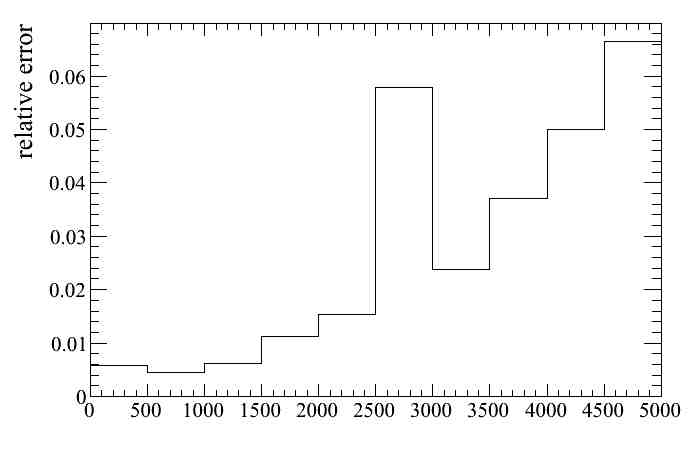
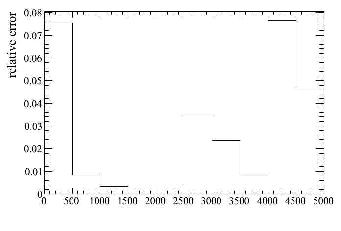
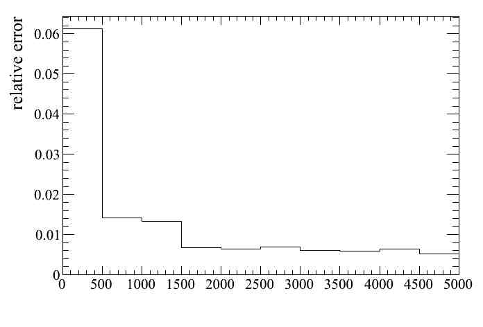
The first plot we can do is a distribution of the relative systematic error as a function of any variable in the micro-tree. For example as a function of the muon candidate momentum for all events passing the numuCC selection.
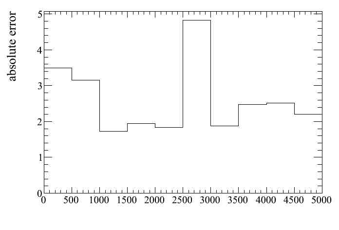
Similarly the absolute error can be ploted.
We can attached systematic error bars to a distribution
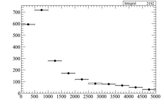
where error bars are only systematics. We have used the root option "e2" in order to make the error bars visible. The total error would be plotted as follows
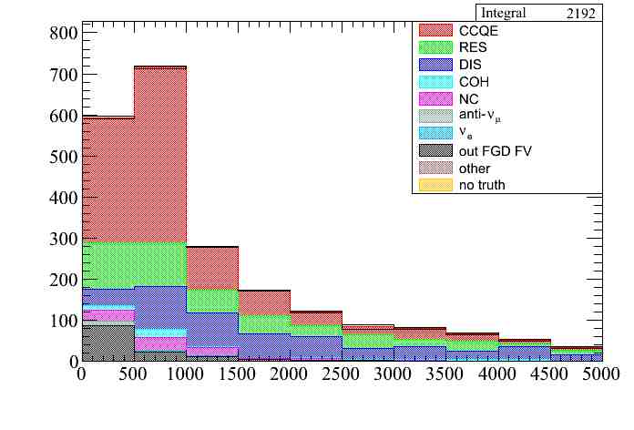
The error can also be plotted when using color plots for a given category using the option "ETOT". In this case the error bar is always a rectangle:
We can now include some weight systematics in our example. Since weight systematics do not modify the event properties and each of them is stored in a different variable in the output tree (weight_syst[i]). we can enable all of them and then plot them independently. The SandMuons systematic is disabled since it should be run over a sand muons file. So we can use this setup in the parameters file.
These are the trees in the output file
Now we can see the list of systematics enabled in the all_syst configuration:
We can plot the relative error for all weight systematics together
Or for some of them, for example OOFV (8) and FGD mass (7):
Finally we can put all systematics together by switching on the variation systematics in the baseTrackerAnalysis parameters file.
Drawing options for systematics
These is the list of options for drawing different systematics:
- SYS: plot all systematics together
- SSYS: plots variation systematics only
- WSYS: plots weight systematics only
- WSYS WS1 WS3: plots weight systematics 1 and 3 only. One can specified any number of weight systematics
- WSYS NWS1 NWS3: plots all weight systematics except 1 and 3. One can exclude any number of weight systematics
- SYS WS1 WS3: plots all variation systematics and weight systematics 1 and 3 only
Notice that individual variation systematics cannot be drawn separately. To do so one should enable a single variation systematic in a given configuration.
Validation of systematic error propagation
How can we be sure that highland is treating correctly the toy experiments for variation systematics ? And how can we be sure that the implementation of a give systematic propagation is correct.
The first question can be answer using the DrawToys functionality of the DrawingTools. The following line draws the distribution of the number of events selected in the 2500-3000 momentum bin for the 10 toy experiments in the "momresol_syst" configuration. This is the bin with abnormal large error shown above. The height of each entry in that plot corresponds to the PDF (gaussian in this case) probability for each of the toys. This is the ana_weight variable in the microtree.
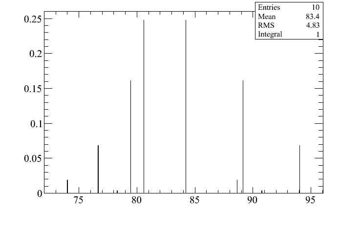
The mean of this plot (83.4) is the number of selected events in that momentum bin, and corresponds to the value in the momentum distribution shown above. The RMS (4.83) is the systematic error and corresponds to the error bar of the momentum distribution shown above, although it can be better checked looking at the absolute error plot.
This only demonstrates the consistency of the different plots in highland. But how can we checked that the momentum resolution error is correctly propagated to the number of selected events (in other words, is the MomentumResolSystematics.cxx correct ?).
This particular systematics has two effects, i) the migration to neighboring bins due to the change in the variable we are plotting (the systematic varies the same variable we are plotting) and ii) the effect on the selection cuts: the muon candidate can change, the PID is affected by the change in momentum, etc.
To check the first we can look at the relative error plot. We realize that as expected the effect of the systematic is larger at large momentum, since the resolution is worst and the momentum bins have the same size. We can increase/decrease the number of bins an check that the relative error increases/decreases. We could even compute analytically the error we expect for a given momentum bin given the resolution at that bin and its width.
On the other hand the second effect is very tiny as we can see by plotting the distribution of toys with no momentum cuts:
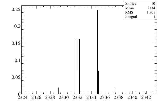
The effect is at the per mil level (1.8/2334).
One should also compare the relative momentum plots with those in technical note 152.
For some weight systematics one would expect a direct connection between the systematic source (numbers in the baseAnalysis/src/systcmatics/data/*.dat files) and the relative systematic error:
- FGDMass, which should be around 0.0067 both in the .dat file and in the plot
- PileUp, which depends on the run period but should be around 0.001 both in the .dat file and in the plot
- TPCFGDMatchEff, which depends on momentum and track multilicity, but for a single selected track above 200 MeV/c should be around 0.0001 both in the .dat file and in the plot
- TPCTrackEff, which should be around 0.004 both in the .dat file and in the plot in topologies with a single track selected