- Introduction
- Setting up the DrawingTools
- Print information on the screen: systematics, cuts, categories, variables ...
- Different plotting functions: 1D, 2D, efficiencies, systematics, data-mc comparisons, etc
- Using DataSample to easily handle multiple data samples
- Using Experiment to easily handle multiple data taking periods
- Configuration for plots: binning, options, style, ...
- Create file with event numbers for a given selection
Introduction
DrawingTools is a highland2 class which can be instanciated from a ROOT session to inspect the output file of a highland2 job and easily understand your analysis. The DrawingTools has methods to dump information about your analysis:
- Which selection(s) was run (see here)
- Which are the available systematics (see here)
- Which systematics were enabled and with how many toy experiments (see here)
- How many POT was processed (see here)
- Which variables are available in the micro-trees and what they are (see here)
- and more (click here to see all available methods)
In this way you may know at any time how a given highland2 output file was built.
But the main functionality of the DrawingTools, at its name suggests, are the tools for drawing. Indeed, the DrawingTools provide all kind of methods to understand the selection and the systematics:
- Draw 1D and 2D distributions, with uniform or variable binning, using a stacked histogram with a breakdown in different categories (true reaction type, topology, particle type, neutrino type, etc), with or without systematic errors (see here)
- Draw the signal efficiency and purity, or the ratio of distributions, as a function of any variable in the tree (see here)
- Understand the evolution of the selection (#events, efficiency, purity) after each cut (see here)
- Compare data with MC with automatic normalization by POT or by area (see here and here)
- Combine in a coherent manner different run periods for data and MC with proper POT normalization (see here)
- Draw the size of the systematic error (total or for individual sources) as a function of any variable (see here)
Setting up the DrawingTools
If you haven't done so yet, you should do under the cmt directory of your top level analysis package:
such that root knows about all important classes in the framework. Then you can open a root session and create a DrawingTools instance with a root file as input:
root -l
root [0] DawingTools draw("file.root");
In this way the DrawingTools will be configured properly using information in the config tree (selection name, cut names, variables description, systematics, corrections, etc). By default the "T2K" plotting style is chosen. If you don't want to use it you can create the DrawingTools instance with a false as second argument
root [1] DawingTools draw("file.root",false);
You can inmediately have a quick look at the cuts that were applied, at the available categories for color code drawing, etc. This file is only used to congigure the DrawingTools. Now if you want to do plots you should either open a root file (could be the same) or create a DataSample intance with a root file as input. This is recomended, since in that case you can easily handle multiple samples (see drawingtools_multi):
Print information on the screen: systematics, cuts, categories, variables ...
Information about variables in the tree
These are the available methods:
void ExplainVar(std::string name, std::string tree_name = "default") {doc().ExplainVar(name, tree_name);}
void ListVars(std::string tree_name = "default") {doc().ListVars(tree_name);}
The following line in the root session
root [4] draw.ExplainVar("accum_level")
produces this output on the screen:
Variable name..... accum_level
Stored in tree.... default
Type of variable.. Vector of integer
Size of variable:
1st dimension... 1 (fixed size)
Documentation..... The number of the first cut that was failed.
highland supports running multiple toys (for evaluating systematics), so the index in this vector is the toy index.
If you only have one toy (normal), then you can use accum_level or accum_level[] to access the correct number.
List of corrections applied
The list of corrections applied in the current output file can be dumped as follows:
root [5] draw.DumpCorrections()
-------- List of Corrections -----------------------------------
#: name enabled applied in input
-----------------------------------------------------------------
0: pileup_corr 1 0
1: tpcdedx_data_corr 1 0
2: tpcdedx_mc_corr 1 0
3: tpcexpecteddedx_corr 1 0
4: ignorerightecal_corr 1 0
5: dq_corr 1 0
-----------------------------------------------------------------
where applied in input means that the input file already had the correction. This will be always false when running over oaAnalysis files, while it will be true in general when running over a FlatTree. When the correction is applied in input it will appear as disabled (not to apply it twice).
List of available systematics
The list of available systematics can be shown as follows:
root [6] draw.DumpSystematics()
-------- List of Systematics --------------------
#: name type NPar
--------------------------------------------------
0: kBFieldDist variation 1
1: kMomScale variation 1
2: kMomResol variation 3
3: kTpcPid variation 104
4: kFgdPid variation 4
5: kChargeConf weight 30
6: kTpcClusterEff weight 2
7: kTpcTrackEff weight 2
8: kTpcFgdMatchEff weight 6
9: kFgdTrackEff weight 14
10: kFgdHybridTrackEff weight 24
11: kMichel weight 8
12: kPileUp weight 7
13: kFgdMass weight 2
14: kOOFV weight 18
15: kSIPion weight 3
16: kSandMu weight 1
17: kFluxWeightNu weight 25
18: kFluxWeightAntiNu weight 25
--------------------------------------------------
Those are the systematics added to the SystematicManager (in the DefineSystematics methods) and not the systematics actually run, since those must be enabled in a specific confifuration, as shown below. The systematic type (variation or weight) and the number of systematic parameters are shown.
List of configurations
A configuration is defined by the list of enabled systematics in a given analysis. The list of configurations can be printed:
root [7] draw.DumpConfigurations()
-------- List of Configurations ----------------------------------
#: name NToys enabled NSyst RandomSeed
-------------------------------------------------------------------
0: default 1 1 0 -1
-------------------------------------------------------------------
There will be a tree with the same name as the configuration in the output file. In this case only the default configuration (allways pressent) was run, with 0 systematics, and no random seed (-1). We can print information about a particular configuration:
root [8] draw.DumpConfiguration("default")
Configuration: default *************
enabled: 1
NToys: 1
NSyst: 0
Random seed: -1
We can repeat the same operations with an output file created with the "all_syst" configuration enabled (baseAnalysis.Configurations.EnableAllSystematics = 1 in baseAnalysis.parameters.dat). In this particular example 9 systematics where enabled in baseAnalysis.parameters.dat, and 100 toy experiments were run:
root [9] draw.DumpConfigurations()
-------- List of Configurations ----------------------------------
#: name NToys enabled NSyst RandomSeed
-------------------------------------------------------------------
0: default 1 1 0 -1
1: all_syst 100 1 9 1
-------------------------------------------------------------------
root [10] draw.DumpConfiguration("all_syst")
Configuration: all_syst *************
enabled: 1
NToys: 100
NSyst: 9
Random seed: 1
-------- List of VariationSystematics ------------
#: name pdf NPar
--------------------------------------------------
0: kMomScale unknown 1
1: kTpcPid unknown 104
--------------------------------------------------
-------- List of WeightSystematics ---------------
#: name pdf NPar
--------------------------------------------------
0: kChargeConf unknown 30
1: kTpcTrackEff unknown 2
2: kMichel unknown 8
3: kPileUp unknown 7
4: kFgdMass unknown 2
5: kOOFV unknown 18
6: kSIPion unknown 3
--------------------------------------------------
In this case the list of systematics enabled in the configuration has been printed. Notice that the pdf (Probability Density Function) is labeled as unknown. This is becouse currently the random numbers for toy experiment variations are thrown externally, so individual systematics do not know its PDF. This will be changed in the future, such that we can know from the output file which pdf was used.
List of selections
The user can print on the screen the list of available selections:
root [11] draw.DumpSelections()
-------- List of Selections --------------------------------------------------------------------------------------------
#: name title enabled force break index in accum_level
-------------------------------------------------------------------------------------------------------------------------
0: kTrackerNumuCC inclusive numuCC selection 1 0 0
-------------------------------------------------------------------------------------------------------------------------
In this particular case only one selection was available and enabled (we have run the numuCCAnalysis). force break with 0 value means that the selection is not stopped when a cut is not pass. This is the standard behavior in highland2 (contrary to running directly in psyche) because we are in general interested in studiying the effect of the different cuts. This behaviour can be modified by changing the input argument in the selection constructor. For example, in highland2/numuCCAnalysis/vXrY/src/numuCCAnalysis.cxx, we find the line:
sel().AddSelection(
"kTrackerNumuCC",
"inclusive numuCC selection",
new numuCCSelection(
false));
To stop the selection when a cut is not passed we should change false by true. The last field printed on the screen index in accum_level is the index of this selection in the accum_level array. When there are several selections in the same analysis the index will be different for each of them such that we can do plots for events that pass a given cut of a given selection.
List of steps and cuts in a selection
The available methods to dump information about steps or cuts in a selection are:
void DumpCuts(int branch=-1);
void DumpSteps(int branch=-1);
void DumpCuts(const std::string& sel_name, int branch=-1);
void DumpSteps(const std::string& sel_name,int branch=-1);
void DumpCuts(Int_t sel_index, int branch);
void DumpSteps(Int_t sel_index,int branch);
In the example below, the numuCCAnalysis was run, which contains a single selection with no branches. In this case we don't have to give any argument to the methods:
root [12] draw.DumpSteps()
-------------------------------------------------------------------
Steps for selection 'kTrackerNumuCC' with no branches
-------------------------------------------------------------------
#: type title break branches
-------------------------------------------------------------------
0: cut event quality 1 0
1: cut > 0 tracks 1 0
2: action find leading tracks 0 0
3: action find vertex 0 0
4: action fill_summary 0 0
5: cut quality+fiducial 1 0
6: action find veto track 0 0
7: cut veto 0 0
8: action find oofv track 0 0
10: cut muon PID 0 0
-------------------------------------------------------------------
root [13] draw.DumpCuts()
-------------------------------------------------------------------
Cuts for selection 'kTrackerNumuCC' with no branches
-------------------------------------------------------------------
#: type title break branches
-------------------------------------------------------------------
0: cut event quality 1 0
1: cut > 0 tracks 1 0
2: cut quality+fiducial 1 0
3: cut veto 0 0
5: cut muon PID 0 0
-------------------------------------------------------------------
For more complicated analysis (with several selections and/or branches) we should specify the selection and the branch.
List of event/track categories
As mentioned above each event has a list of categories associated, which are in general related with the true properties of the event. For example one can plot the momentum distribution of the muon candidate with different colors for each particle type (stacked histogram). In this way we can see how many of our selected muons are in fact true muons. To do so the user have to specify the "particle" category in the corresponding DrawingTools method. There are other categories as true reaction type, detector in which the true interaction happened, etc. The list of categories or info about a specific category can be accessed using the following methods:
void DumpCategories(){cat().DumpCategories();}
void DumpCategories(const std::string& file){ReadCategories(file);cat().DumpCategories();if (_config_file!="") ReadCategories(_config_file);}
void DumpCategory(std::string category) {cat().DumpCategory(category);}
The list of categories:
root [14] draw.DumpCategories()
-------- Available track categories -------
- particle
- parent
- gparent
- primary
- nutype
- detector
- target
- reaction
- reactionCC (=1 when reaction<4 || reaction==9 for 2p2h)
- reactionnofv
- reactionsand
- reactionsandCC
- topology
- topology_no1pi
- topology_withpi0
- topology_ccpizero
- mectopology
-------- Track categories
for FGD2 (
if defined) -------
- fgd2<one_of_the_previous>
-------- Track categories for antinu (if defined) -------
same names as previous
-------------------------------------------
As mentioned above, there is also a method to print the available types for a given category, including the details (color, code) for each type:
root [14] draw.DumpCategory("reaction")
-------- Types for 'reaction' category -------
- CCQE (code 0, color 2)
- 2p2h (code 9, color 874)
- RES (code 1, color 3)
- DIS (code 2, color 4)
- COH (code 3, color 7)
- NC (code 4, color 6)
- anti-#nu_{#mu} (code 5, color 31)
- #nu_{e} (code 6, color 65)
- out FGD FV (code 7, color 1)
- other (code 999, color 48)
- no truth (code -1, color 92)
-------------------------------------------
POT information
Information about the POT corresponding to the data being analyses can be accessed with several methods. The simplest options are:
void DumpPOT(TTree* tree);
void DumpPOT(const std::string& file);
These are the available methods using DataSample or Experiment:
void DumpPOT(
Experiment& exp,
const std::string& samplegroup_name);
double GetNormalisationFactor(
DataSample* sample1,
DataSample* sample2,
double norm=-1.,
bool pot_norm=
true,
const std::string& opt=
"");
This is one example for a single MC file:
root [16] draw.DumpPOT(mc)
Initial POT........... 5e+17
|-- Bad Beam.......... 0
|-- Bad ND280......... 0
|-- Total Good POT.... 5e+17
|-- @ 0KA........... 0
|-- @ 200KA......... 0
|-- @ 250KA......... 0
|-- @ Other power... 0
Purities
void PrintPurities(TTree* tree, const std::string& categ, const std::string& cut);
Produces the following output on the screen:
root [15] draw.PrintPurities(default,"reaction","accum_level>5")
Purities
Category reaction
Cut accum_level>5
Events 50283.6
------------------------------------------
CCQE 44.2077 % (22229.2 events)
2p2h 0 % (0 events)
RES 22.4987 % (11313.2 events)
DIS 20.7072 % (10412.3 events)
COH 2.84522 % (1430.68 events)
NC 3.2865 % (1652.57 events)
anti-#nu_{#mu} 0.577795 % (290.536 events)
#nu_{e} 0.295568 % (148.622 events)
out FGD FV 5.53933 % (2785.37 events)
other 0.0467397 % (23.5024 events)
no truth 0 % (0 events)
------------------------------------------
In this particular case the 2p2h category has 0 events becaouse the job was run on production 5 files.
If your microtree has more than one branch or selection, replace accum_level as explained in the next paragraph.
Different plotting functions: 1D, 2D, efficiencies, systematics, data-mc comparisons, etc
The DrawingTools have the following drawing functionality:
The functions shown below are in the class DrawingToolsBase.
In the follwing examples it is used a microtree with just one branch and one selection. For extending to a general case just replace: for microtrees with more than one branch OR more than one selection but without any branches: for functions on the truth tree: accum_level –> accum_level[branchID or selectionID] for functions on the default tree: accum_level –> accum_level[][branchID or selectionID] (the first empty [] is for the toy experiment) for microtrees with more than one selection AND more than one branches: for functions on the truth tree: accum_level –> accum_level[selectionID][branchID] for functions on the default tree: accum_level –> accum_level[][selectionID][branchID] (the first empty [] is for the toy experiment)
There are methods to draw single 1D or 2D distributions, provided the variable(s), the binning, the category to be plotted and the cut:
Draw single distributions
void Draw(TTree* tree, const std::string& var, int nx, double xmin, double xmax, const std::string& categ="all",
const std::string& cut="", const std::string& root_opt="", const std::string& opt="", double norm=1,bool scale_errors=true);
void Draw(TTree* tree, const std::string& var, int nx, double xmin, double xmax, int ny, double ymin, double ymax,
const std::string& categ="all", const std::string& cut="", const std::string& root_opt="", const std::string& opt="", double norm=1,bool scale_errors=true);
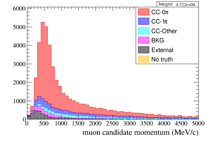
For example, a typical 1D distribution is:
root [16] draw.SetTitleX("muon candidate momentum (MeV/c)")
root [17] draw.Draw(default,"selmu_mom",50,0,5000,"topology","accum_level>5")
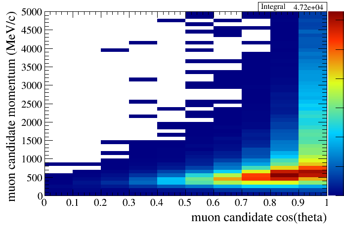
The syntax for drawing 2D plots follows ROOT's convention. The string you pass as the var option should be of the form
You can read this as plot y_var as a function of x_var. As an example of 2D distribution:
root [18] draw.SetTitleX("muon candidate cos(theta)")
root [19] draw.SetTitleY("muon candidate momentum (MeV/c)")
root [20] draw.Draw(default,"selmu_mom:selmu_costheta",10,0,1,50,0,5000,"all","accum_level>5","colz")
The 'cut' argument
The cut argument will normally just be used to select events passing a given cut, such as
However, this can be any cut string that ROOT supports. You can reference any variable stored in the micro-tree, so could do something like this to only look at events passing the first 3 cuts and that have a momentum greater than 300 MeV (assuming your momentum variable is called selmu_mom).
"accum_level>2 && selmu_mom>300"
The same applies to the var argument, where you can combine multiple variables into a single one.
Vector and matrix variables
If you have saved vector variables in your output tree, for example to save a direction as a 3D array, you can access the components of the vector using the following syntax:
The argument in square brackets denotes the element of the vector you are accessing. You can combine vector variables and 2D plots to create, for example, 2D distributions of where interactions occur, using
which will create an X-Y plot. To make this pretty, you should pass "COLZ" as the root_opt argument when callign Draw().
You can also store matrix variables (with two indices) and 3D matrix variables (with three indices). The way of plotting those variables is similar to vectors, but you should specify the appropriate number of indices.
Imagine you have the position of all tpc segements in your muon candidate stored as matrix variable (selmu_tpc_pos), in which the first index corresponds to a given TPC and the second index to the component of the position. If you want to plot the y position of the first TPC you should use:
If on the contrary you want to plot the y position for all tpc segments:
where the empty brackets is interpreted by ROOT and "all" components. A similar format is used for 3D matrix variables. You can use combinations as:
"var[][][2]"
"var[1][][2]"
"var[][1][2]"
"var[1][1][2]"
Draw ratios, efficiencies, purities and significances
These are the available methods, both for uniform and variable binning:
void DrawRatio(TTree* tree, const std::string& var, int nbins, double* xbins,
const std::string& cut1, const std::string& cut2, const std::string& root_opt="", const std::string& opt="", const std::string& leg="");
void DrawRatio(TTree* tree, const std::string& var, int nx, double xmin, double xmax,
const std::string& cut1, const std::string& cut2, const std::string& root_opt="", const std::string& opt="", const std::string& leg="");
void DrawEff(TTree* tree, const std::string& var, int nbins, double* xbins, const std::string& cut1, const std::string& cut2,
const std::string& root_opt="", const std::string& opt="", const std::string& leg="");
void DrawEff(TTree* tree, const std::string& var, int nx, double xmin, double xmax, const std::string& cut1, const std::string& cut2,
const std::string& root_opt="", const std::string& opt="", const std::string& leg="");
void DrawDoubleEff(TTree* tree1, TTree* tree2, const std::string& var, int nx, double* xbins,
const std::string& cut1, const std::string& cut2, const std::string& root_opt="", const std::string& opt="", const std::string& leg="");
void DrawDoubleEff(TTree* tree1, TTree* tree2, const std::string& var, int nx, double xmin, double xmax,
const std::string& cut1, const std::string& cut2, const std::string& root_opt="", const std::string& opt="", const std::string& leg="");
void DrawSignificance(TTree* tree, const std::string& var, int nbins, double* xbins, const std::string& cut1, const std::string& cut2,
double norm=1, double rel_syst=0,const std::string& root_opt="", const std::string& opt="", const std::string& leg="");
void DrawSignificance(TTree* tree, const std::string& var, int nbins, double xmin, double xmax, const std::string& cut1, const std::string& cut2,
double norm=1, double rel_syst=0,const std::string& root_opt="", const std::string& opt="", const std::string& leg="");
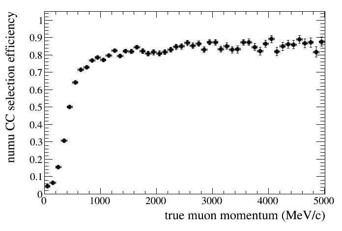
For example we can draw the selection efficiency using the truth tree. In this example the denominator will contain all true numu CC events while the numerator will contain all true numu CC events that are selected:
root [18] draw.SetTitleX("true muon momentum (MeV/c)")
root [19] draw.SetTitleY("numu CC selection efficiency")
root [20] draw.DrawEff(truth,"truemu_truemom",50,0,5000,"accum_level>5","reactionCC==1")
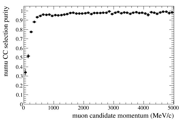
And the selection purity using the default tree. In this case we use the same method but exchange the cut order. The denominator will contain all selected events while the numerator will contsin all selected events that are true numu cc.
draw.SetTitleX("muon candidate momentum (MeV/c)")
draw.SetTitleY("numu CC selection purity")
draw.DrawEff(default,"selmu_mom",50,0,5000,"reactionCC==1","accum_level>5")
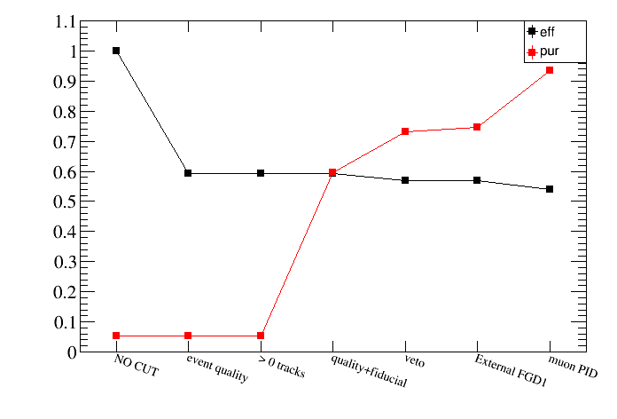
Draw number of events, efficiency and purity as a function of the cut
These are the available methods:
void DrawEventsVSCut(TTree* tree, const std::string& cut_norm="", int first_cut=-1, int last_cut=-1,
const std::string& root_opt="", const std::string& opt="", const std::string& leg="");
void DrawEventsVSCut(TTree* tree, int branch, const std::string& cut_norm="", int first_cut=-1, int last_cut=-1,
const std::string& root_opt="", const std::string& opt="", const std::string& leg="");
void DrawEventsVSCut(TTree* tree, int isel, int branch, const std::string& cut_norm="", int first_cut=-1, int last_cut=-1,
const std::string& root_opt="", const std::string& opt="", const std::string& leg="");
void DrawRatioVSCut(TTree* tree1, TTree* tree2, const std::string& precut="", int first_cut=-1, int last_cut=-1,
const std::string& root_opt="", const std::string& opt="", const std::string& leg="", double norm=1.);
void DrawRatioVSCut(TTree* tree1, TTree* tree2, int branch, const std::string& precut="", int first_cut=-1, int last_cut=-1,
const std::string& root_opt="", const std::string& opt="", const std::string& leg="", double norm=1.);
void DrawRatioVSCut(TTree* tree1, TTree* tree2, int isel, int branch, const std::string& precut="", int first_cut=-1, int last_cut=-1,
const std::string& root_opt="", const std::string& opt="", const std::string& leg="", double norm=1.);
void DrawEffVSCut(TTree* tree, const std::string& signal="", const std::string& precut="", int first_cut=-1, int last_cut=-1,
const std::string& root_opt="", const std::string& opt="", const std::string& leg="");
void DrawEffVSCut(TTree* tree, int branch, const std::string& signal="", const std::string& precut="", int first_cut=-1, int last_cut=-1,
const std::string& root_opt="", const std::string& opt="", const std::string& leg="");
void DrawEffVSCut(TTree* tree, int isel, int branch, const std::string& signal="", const std::string& precut="", int first_cut=-1, int last_cut=-1,
const std::string& root_opt="", const std::string& opt="", const std::string& leg="");
void DrawPurVSCut(TTree* tree, const std::string& signal="", const std::string& precut="", int first_cut=-1, int last_cut=-1,
const std::string& root_opt="", const std::string& opt="", const std::string& leg="");
void DrawPurVSCut(TTree* tree, int branch, const std::string& signal="", const std::string& precut="", int first_cut=-1, int last_cut=-1,
const std::string& root_opt="", const std::string& opt="", const std::string& leg="");
void DrawPurVSCut(TTree* tree, int isel, int branch, const std::string& signal="", const std::string& precut="", int first_cut=-1, int last_cut=-1,
const std::string& root_opt="", const std::string& opt="", const std::string& leg="");
All those methods exist also for DataSample. There are other methods, which take two DataSamples:
void DrawRatioVSCut(
DataSample& sample1,
DataSample& sample2,
const std::string& precut=
"",
int first_cut=-1,
int last_cut=-1,
const std::string& root_opt="", const std::string& opt="", const std::string& leg="", double norm=-1., bool pot_norm=true);
void DrawRatioVSCut(
DataSample& sample1,
DataSample& sample2,
int branch,
const std::string& precut=
"",
int first_cut=-1,
int last_cut=-1,
const std::string& root_opt="", const std::string& opt="", const std::string& leg="", double norm=-1., bool pot_norm=true);
void DrawRatioVSCut(
DataSample& sample1,
DataSample& sample2,
int isel,
int branch,
const std::string& precut=
"",
int first_cut=-1,
int last_cut=-1,
const std::string& root_opt="", const std::string& opt="", const std::string& leg="", double norm=-1., bool pot_norm=true);
void DrawEffPurVSCut(
DataSample& sample,
const std::string& signal,
const std::string& precut=
"",
int first_cut=-1,
int last_cut=-1,
const std::string& root_opt="", const std::string& opt="", const std::string& leg="");
void DrawEffPurVSCut(
DataSample& sample,
int branch,
const std::string& signal,
const std::string& precut=
"",
int first_cut=-1,
int last_cut=-1,
const std::string& root_opt="", const std::string& opt="", const std::string& leg="");
void DrawEffPurVSCut(
DataSample& sample,
int isel,
int branch,
const std::string& signal,
const std::string& precut=
"",
int first_cut=-1,
int last_cut=-1,
const std::string& root_opt="", const std::string& opt="", const std::string& leg="");
void DrawEffPurVSCut(
DataSample& sample,
int isel,
int branch,
const std::string& signal,
const std::string& precut,
int first_cut_pur, int last_cut_pur, int first_cut_eff, int last_cut_eff,
const std::string& root_opt="", const std::string& opt="", const std::string& leg="");
And here some examples:
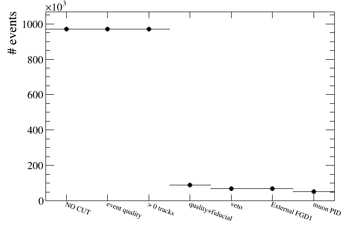
root [21] draw.DrawEventsVSCut(default)
As you can see the first two cuts have no effect because we only saved in the micro-tree events with accum_level>2 (SetMinAccumLevelToSave). We can remove those cuts from the plot as follows:
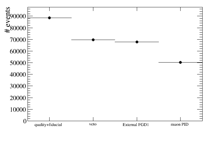
root [22] draw.DrawEventsVSCut(default,"",2)
what means that only cuts starting from cut number 2 (quality+fiducial) will be shown:
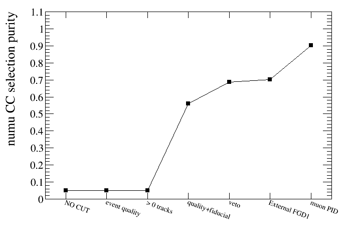
root [23] draw.SetTitleY("numu CC selection purity")
root [24] draw.DrawPurVSCut(default,"reactionCC==1")
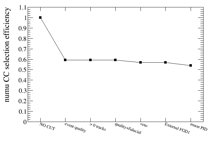
root [25] draw.SetTitleY("numu CC selection efficiency")
root [26] draw.DrawEffVSCut(truth,"reactionCC==1")
The example below needs a DataSample to handle simultaneously the default and truth trees. More information about DataSample can be found below
root [28] draw.SetTitleY("")
root [29] draw.DrawEffPurVSCut(mc,"reactionCC==1")
Drawing statistical and systematic errors
A detailed description of systematic errors and how to draw them can be found an the systematics page. Here we just list the available drawing methods.
To plot relative or absolute errors as a faction of any variable:
Double_t DrawErrors(TTree* tree, const std::string& var, int nx, double xmin, double xmax,
const std::string& cut="", const std::string& root_opt="", const std::string& opt="", const std::string& leg="", double norm=1, bool scale_errors=false);
Double_t DrawRelativeErrors(TTree* tree, const std::string& var, int nx, double xmin, double xmax,
const std::string& cut="", const std::string& root_opt="", const std::string& opt="", const std::string& leg="", double norm=1, bool scale_errors=false);
Double_t DrawErrors(TTree* tree, const std::string& var, int nx, double* xbins,
const std::string& cut="", const std::string& root_opt="", const std::string& opt="", const std::string& leg="", double norm=1, bool scale_errors=false);
Double_t DrawRelativeErrors(TTree* tree, const std::string& var, int nx, double* xbins,
const std::string& cut="", const std::string& root_opt="", const std::string& opt="", const std::string& leg="", double norm=1, bool scale_errors=false);
Double_t DrawRelativeErrors(TTree* tree1, TTree* tree2, const std::string& var, int nx, double xmin, double xmax,
const std::string& cut="", const std::string& root_opt="", const std::string& opt="", const std::string& leg="", double norm=1, bool scale_errors=false);
Double_t DrawRelativeErrors(TTree* tree1, TTree* tree2, const std::string& var, int nx, double* xbins,
const std::string& cut="", const std::string& root_opt="", const std::string& opt="", const std::string& leg="", double norm=1, bool scale_errors=false);
Double_t DrawErrors(
Experiment& exp,
const std::string& groupName,
const std::string& mcSampleName,
const std::string& var,
int nx,
double xmin,
double xmax,
const std::string& cut="", const std::string& root_opt="", const std::string& opt="", const std::string& leg="", bool scale_errors=false);
Double_t DrawRelativeErrors(
Experiment& exp,
const std::string& groupName,
const std::string& mcSampleName,
const std::string& var,
int nx,
double xmin,
double xmax,
const std::string& cut="", const std::string& root_opt="", const std::string& opt="", const std::string& leg="", bool scale_errors=false);
Double_t DrawErrors(
Experiment& exp,
const std::string& groupName,
const std::string& mcSampleName,
const std::string& var,
int nx,
double* xbins,
const std::string& cut="", const std::string& root_opt="", const std::string& opt="", const std::string& leg="", bool scale_errors=false);
Double_t DrawRelativeErrors(
Experiment& exp,
const std::string& groupName,
const std::string& mcSampleName,
const std::string& var,
int nx,
double* xbins,
const std::string& cut="", const std::string& root_opt="", const std::string& opt="", const std::string& leg="", bool scale_errors=false);
Double_t DrawErrors(
Experiment& exp,
const std::string& var,
int nx,
double xmin,
double xmax,
const std::string& cut="", const std::string& root_opt="", const std::string& opt="", const std::string& leg="", bool scale_errors=false);
Double_t DrawRelativeErrors(
Experiment& exp,
const std::string& var,
int nx,
double xmin,
double xmax,
const std::string& cut="", const std::string& root_opt="", const std::string& opt="", const std::string& leg="", bool scale_errors=false);
Double_t DrawErrors(
Experiment& exp,
const std::string& var,
int nx,
double* xbins,
const std::string& cut="", const std::string& root_opt="", const std::string& opt="", const std::string& leg="", bool scale_errors=false);
Double_t DrawRelativeErrors(
Experiment& exp,
const std::string& var,
int nx,
double* xbins,
const std::string& cut="", const std::string& root_opt="", const std::string& opt="", const std::string& leg="", bool scale_errors=false);
We can select statistical errors, systematics or both using the appropriate options (see the options Options for Drawing methods). If no option is given statistical errors will be plotted. We can also draw the covariance matrix:
void DrawCovMatrix(TTree* tree, const std::string& var, int nx, double xmin, double xmax,
const std::string& cut="", const std::string& root_opt="", const std::string& uopt="");
void DrawCovMatrix(TTree* tree, const std::string& var, int nx, double* xbins,
const std::string& cut="", const std::string& root_opt="", const std::string& uopt="");
void DrawCovMatrix(
Experiment& exp,
const std::string& groupName,
const std::string& mcSampleName,
const std::string& var,
int nx,
double* xbins,
const std::string& cut="", const std::string& root_opt="", const std::string& uopt="");
void DrawCovMatrix(
Experiment& exp,
const std::string& groupName,
const std::string& mcSampleName,
const std::string& var,
int nx,
double xmin,
double xmax,
const std::string& cut="", const std::string& root_opt="", const std::string& uopt="");
void DrawCovMatrix(
Experiment& exp,
const std::string& var,
int nx,
double* xbins,
const std::string& cut="", const std::string& root_opt="", const std::string& uopt="");
void DrawCovMatrix(
Experiment& exp,
const std::string& var,
int nx,
double xmin,
double xmax,
const std::string& cut="", const std::string& root_opt="", const std::string& uopt="");
const TMatrixD& GetCovMatrix(TTree* tree, const std::string& var, int nx, double* xbins,
const std::string& cut="", const std::string& uopt="");
const TMatrixD& GetCovMatrix(TTree* tree, const std::string& var, int nx, double xmin, double xmax,
const std::string& cut="", const std::string& uopt="");
const TMatrixD& GetCovMatrix(
Experiment& exp,
const std::string& groupName,
const std::string& mcSampleName,
const std::string& var,
int nx,
double xmin,
double xmax,
const std::string& cut="", const std::string& root_opt="", const std::string& uopt="");
const TMatrixD& GetCovMatrix(
Experiment& exp,
const std::string& groupName,
const std::string& mcSampleName,
const std::string& var,
int nx,
double* xbins,
const std::string& cut="", const std::string& root_opt="", const std::string& uopt="");
const TMatrixD& GetCovMatrix(
Experiment& exp,
const std::string& var,
int nx,
double xmin,
double xmax,
const std::string& cut="", const std::string& root_opt="", const std::string& uopt="");
const TMatrixD& GetCovMatrix(
Experiment& exp,
const std::string& var,
int nx,
double* xbins,
const std::string& cut="", const std::string& root_opt="", const std::string& uopt="");
Toy experiments plots
In addition to the methods above to draw systematic errors there are methods to check the distribution of toy experiments:
void DrawToys(TTree* tree, const std::string& cut="", const std::string& root_opt="", const std::string& opt="", const std::string& leg="");
void DrawToysRatio(TTree* tree1, TTree* tree2, const std::string& cut="",
const std::string& root_opt="", const std::string& opt="", const std::string& leg="", double norm=1);
void DrawToysRatioTwoCuts(TTree* tree1, TTree* tree2, const std::string& cut1, const std::string& cut2,
const std::string& root_opt="", const std::string& opt="", const std::string& leg="",double norm=1);
Comparison between two data samples
In this case either you open two root files containg the output of two different analyses for two data samples (data.root, mc.root), and copy simultaneously in memory the micro-trees we want a use to compare, or use DataSample, which handles multiple data samples for you (see below)
void Draw(TTree* tree1, TTree* tree2, const std::string& var, int nx, double xmin, double xmax,
const std::string& categ="all", const std::string& cut="", const std::string& root_opt="", const std::string& opt="", double norm=1,
void Draw(TTree* tree1, TTree* tree2, const std::string& var, int nx, double xmin, double xmax, int ny, double ymin, double ymax,
const std::string& categ="all", const std::string& cut="",
const std::string& root_opt="", const std::string& opt="", double norm=1, bool scale_errors=false);
void DrawRatio(TTree* tree1, TTree* tree2, const std::string& var, int nx, double xmin, double xmax,
const std::string& cut="", const std::string& root_opt="", const std::string& opt="", const std::string& leg="", double norm=1);
void DrawRatioTwoCuts(TTree* tree1, TTree* tree2, const std::string& var, int nx, double xmin, double xmax,
const std::string& cut1, const std::string& cut2,
const std::string& root_opt="", const std::string& opt="", const std::string& leg="", double norm=1);
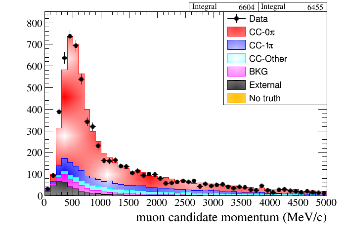
Using DataSample to easily handle multiple data samples
All functions above are also available using DataSample as input instead of a single tree. For example for a data-MC comparison:
void Draw(
DataSample& sample1,
DataSample& sample2,
const std::string& var,
int nx,
double xmin,
double xmax,
const std::string& categ="all", const std::string& cut="",
const std::string& root_opt="", const std::string& opt="",bool scale_errors=false, double norm=1, bool pot_norm=true);
where sample1 and sample 2 will be created using two different micro-tree files (output of highland analyses):
In this case the normalization factor will be computed automatically (unless we specify the contrary in the last argument) from the header tree in both DataSample. Those extended functions are part of DrawingTools, which inherits from DrawingToolsBase. The code and figure below show an example:
root [4] draw.SetTitleX("muon candidate momentum (MeV/c)")
root [5] draw.Draw(data,mc,"selmu_mom",50,0,5000,"topology","accum_level>5")
Now we list all available methods for samples comparison:
void Draw(
DataSample& sample1,
DataSample& sample2,
const std::string& var,
int nx,
double xmin,
double xmax,
const std::string& categ="all", const std::string& cut="",
const std::string& root_opt="", const std::string& opt="", double norm=1, bool scale_errors=false, bool pot_norm=true);
void Draw(
DataSample& sample1,
DataSample& sample2,
const std::string& var,
int nx,
double xmin,
double xmax,
int ny,
double ymin,
double ymax,
const std::string& categ="all", const std::string& cut="",
const std::string& root_opt="", const std::string& opt="", double norm=1, bool scale_errors=false, bool pot_norm=true);
void DrawRatioTwoCuts(
DataSample& sample1,
DataSample& sample2,
const std::string& var,
int nx,
double xmin,
double xmax,
const std::string& cut1, const std::string& cut2,
const std::string& root_opt="", const std::string& opt="", const std::string& leg_name="", double norm=1, bool pot_norm=true);
void DrawRatio(
DataSample& sample1,
DataSample& sample2,
const std::string& var,
int nx,
double xmin,
double xmax,
const std::string& cut="",
const std::string& root_opt="", const std::string& opt="", const std::string& leg_name="", double norm=1, bool pot_norm=true);
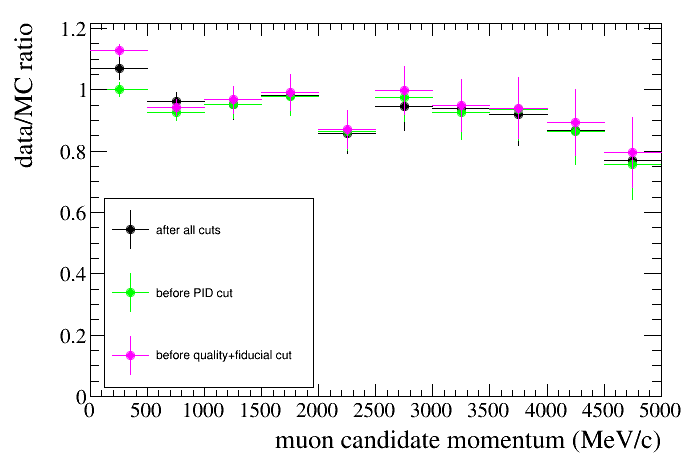
The plot below shows the data/MC ratio as a function of the muon candidate momentum for different cuts. Here we also learn how to change the legend position to the bottom-left ("bl") corner:
root [9] draw.SetLegendPos("bl")
root [9] draw.SetTitleX("muon candidate momentum (MeV/c)")
root [8] draw.SetTitleY("data/MC ratio")
root [6] draw.DrawRatio(data,mc,"selmu_mom",10,0,5000,"accum_level>5","","","after all cuts")
root [7] draw.DrawRatio(data,mc,"selmu_mom",10,0,5000,"accum_level>4","same","","before PID cut")
root [7] Draw.DrawRatio(data,mc,"selmu_mom",10,0,5000,"accum_level>2","same","","before quality+fiducial cut")
Data MC comparison plots can be also done using the Experiment class (see below).
Using Experiment to easily handle multiple data taking periods
The Experiment class allows to make data-MC comparison plots with separated data-MC sample pairs for each data taking period, taking into account the proper POT normalization between data and MC for each run.
We can define an Experiment as a collection of SampleGroup's, where each sample group would correspond to a different data taking period. A SampleGroup would contain several samples (DataSample), one for real data and several for MC ("magnet", "sand", etc). The code below creates an Experiment, suitable for nd280 data:
run1.AddDataSample(data1);
run1.AddMCSample("magnet",mc1);
run1.AddMCSample("sand",sand1);
run2w.AddDataSample(data2w);
run2w.AddMCSample("magnet",mc2w);
run2w.AddMCSample("sand",sand2w);
run2a.AddDataSample(data2a);
run2a.AddMCSample("magnet",mc2a);
run2a.AddMCSample("sand",sand2a);
run3.AddDataSample(data3);
run3.AddMCSample("magnet",mc3);
run3.AddMCSample("sand",sand3);
run4.AddDataSample(data4);
run4.AddMCSample("magnet",mc4);
run4.AddMCSample("sand",sand4);
exp.AddSampleGroup("run1", run1);
exp.AddSampleGroup("run2w",run2w);
exp.AddSampleGroup("run2a",run2a);
exp.AddSampleGroup("run3", run3);
exp.AddSampleGroup("run4", run4);
Once the Experiment is defined plots can be made:
void Draw(
Experiment& exp,
const std::string& var,
int nx,
double xmin,
double xmax,
const std::string& categ="all", const std::string& cut="", const std::string& root_opt="", const std::string& opt="",bool scale_errors=false);
void Draw(
Experiment& exp,
const std::string& groupName,
const std::string& var,
int nx,
double xmin,
double xmax,
const std::string& categ="all", const std::string& cut="", const std::string& root_opt="", const std::string& opt="",bool scale_errors=false);
void Draw(
Experiment& exp,
const std::string& groupName,
const std::string& mcSampleName,
const std::string& var,
int nx,
double xmin,
double xmax,
const std::string& categ="all", const std::string& cut="", const std::string& root_opt="", const std::string& opt="",bool scale_errors=false);
In the later two functions, groupName and mcSampleName can take the value "all". For example
root [6] draw.Draw(exp,"run2w","sand","selmu_mom",50,0,5000,"reaction","accum_level>5")
would plot Run 2 water for data and the corresponding sand muon MC only properly normalized, while
root [7] draw.Draw(exp,"all","sand","selmu_mom",50,0,5000,"reaction","accum_level>5")
would plot all data runs and the corresponding sand muon MC only properly normalized for each run.
Configuration for plots: binning, options, style, ...
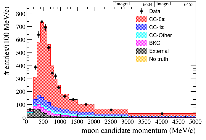
Variable binning
All functions above for which binning should be specified have the corresponding function with variable binning. In that case
int nx, double xmin, double xmax
should be substituded by
and
int nx, double xmin, double xmax , int ny, double ymin, double ymax
should be substituded by
int nx, double* xbins, int ny, double* ybins
For example:
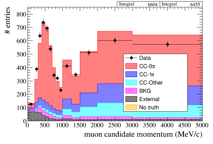
root [8] draw.SetTitleX("muon candidate momentum (MeV/c)")
root [9] draw.SetTitleY("# entries / (100 MeV/c)")
root [10] double pbins[15] = {0, 200, 300, 400, 500, 600, 700, 800, 900, 1000, 1250, 1500, 2000, 3000, 5000};
root [11] draw.Draw(data,mc,"selmu_mom",14,pbins,"topology","accum_level>5")
produces the following plot:
By default, to keep a nice plot appearence, bin contents are normalized to the bin width. If we want disable that feature we should use the option "NOVARBIN":
root [12] draw.SetTitleY("# entries")
root [13] draw.Draw(data,mc,"selmu_mom",14,pbins,"topology","accum_level>5",1,"","NOVARBIN")
Options for Drawing methods
Most functions described above take the following arguments:
- root_opt: this is the standard ROOT plotting option. Options such as "same", "e1", ..., should be specified here
- opt: this is the DrawingTools option. They are described below.
- leg: In some cases you can include a legend in the plots. If you use the root_opt "same" you can superimposed several plots with different legends
The list of DrawingTools options can be printed on the screen with the command:
root [14] draw.ListOptions()
The available options are defined in the DrawingUtils.cxx file:
drawUtils::AddOption(
"SCALETODATA",
"Scale the MC covariance matrix to data POT when using Experiment");
drawUtils::AddOption(
"E0",
"Error style option for second sample. Does the same as the root option e0");
drawUtils::AddOption(
"E1",
"Error style option for second sample. Does the same as the root option e1");
drawUtils::AddOption(
"E2",
"Error style option for second sample. Does the same as the root option e2");
drawUtils::AddOption(
"E3",
"Error style option for second sample. Does the same as the root option e3");
drawUtils::AddOption(
"E4",
"Error style option for second sample. Does the same as the root option e4");
drawUtils::AddOption(
"E5",
"Error style option for second sample. Does the same as the root option e5");
drawUtils::AddOption(
"E6",
"Error style option for second sample. Does the same as the root option e6");
drawUtils::AddOption(
"ETOT",
"When drawing with color codes, draw also the total error for the stacked histogram");
drawUtils::AddOption(
"NOTOTERROR",
"Don't draw the total error (stat+syst) but only the statistical or systematic error");
drawUtils::AddOption(
"NOSTERROR",
"Don't draw the statistical error but only the total error, and also the systematic error when SYSTERROR options is also used");
drawUtils::AddOption(
"SYSTERROR",
"Don't draw the statistical error but only the systematic error, together with the total");
drawUtils::AddOption(
"NODRAW",
"Don't draw anything. You should use the option DUMP to see the results");
drawUtils::AddOption(
"ST",
"When using DrawErrors or DrawRelativeErrors only statistical errors are plotted. In combination with SYS, SSYS or WSYS adds statisticak and systematic errors in quadrature");
drawUtils::AddOption(
"SYS",
"draw all systematics. Error bars correspond to the RMS of all toy experiments");
drawUtils::AddOption(
"SSYS",
"Draw only standard systematics (reconstructed observable variations)");
drawUtils::AddOption(
"WSi",
"Draw only the specified (ith) weight systematic(s) (\" WS0 WS3 ... \")");
drawUtils::AddOption(
"NWSi",
"Exclude the specified (ith) weight systematic(s) (\"NWS0 NWS1 ... \")");
drawUtils::AddOption(
"WCi",
"Draw only the specified (ith) weight correction(s) (\" WC0 WC3 ... \")");
drawUtils::AddOption(
"NWCi",
"Exclude the specified (ith) weight correction(s) (\"NWC0 NWC1 ... \")");
drawUtils::AddOption(
"RELATIVE",
"When computing the covariance matrix divide by the average in each bin such that a relative covariance is computed");
drawUtils::AddOption(
"EFF",
"The efficiency-like ratio plot (out of two histograms, pass and total) is drawn, internal option");
drawUtils::AddOption(
"NOVARBIN",
"Plotting with variable binning, bin entries are normalized by bin width. This option disables this feature.");
drawUtils::AddOption(
"NOTOYW",
"No toy weight is applied for toy experiments. All toys will have the same weight 1.");
drawUtils::AddOption(
"NODEFAULT",
"By default the -999 default is plotted unless this option is used");
drawUtils::AddOption(
"AREA",
"For 1D histos normalization to 1 (if there is only one sample) or to the area of the first sample. In this normalization procedure the whole range of the variable allowed by 'cut' parameter is taken into account");
drawUtils::AddOption(
"AREA1",
"For 1D histos normalization to 1. In this normalization procedure the whole range of the variable allowed by 'cut' parameter is taken into account");
drawUtils::AddOption(
"AREA100",
"For 1D histos normalization to 100. In this normalization procedure the whole range of the variable allowed by 'cut' parameter is taken into account");
drawUtils::AddOption(
"POTNORM",
"Normalize the MC to the POT given as input normalization factor, regardless of the data POT (interprete valid norm factor as a POT value)");
drawUtils::AddOption(
"DRAWALLMC",
"Draw with black contour a histogram for all MC entries (works only while plotting histogram stack)");
drawUtils::AddOption(
"DRAWALLCUTS",
"Draw all cuts even if they are below the MinAccumLevelToSave when doing plots VSCuts");
drawUtils::AddOption(
"NOINFO",
"Dont dump on the screen histogram info when using the Draw methods");
Explaination of a specific option can be printed as follows:
root [13] draw.ExplainOption("PUR")
PUR: The purity is printed on the screen
Notice that several options can be combined. For example "ST SYS" will plot error bars as the sum in quadrature of statistical and systematic errors.
Command line style options
You can change the plot appearence by changing several attributes, such that the position of the legend, the X and Y labels, etc. Once a given attribute is set it will have effect on all subsequent plots. This are the available methods:
void SetLegendEntryHeight(double h){drawUtils::legendEntryHeight=h;}
void SetLegendParam(double a, double b, double c, double d);
void SetLegendPos(double x=-999, double y=-999);
void SetLegendPos(std::string pos);
void SetLegendSize(double w = -999, double h = -999);
void SetSmallLegendSize(double w = -999, double h = -999){if (w != -999) _legendSmallSize[0] = w; if (h != -999) _legendSmallSize[1] = h;}
double GetLegendX() { return _legendPos[0]; }
double GetLegendY() { return _legendPos[1]; }
double GetLegendW() { return _legendSize[0]; }
double GetLegendH() { return _legendSize[1]; }
double GetSmallLegendX() { return _legendPos[0]+_legendSize[0]-_legendSmallSize[0]; }
double GetSmallLegendY() { return _legendPos[1]+_legendSize[1]-_legendSmallSize[1]; }
double GetSmallLegendW() { return _legendSmallSize[0]; }
double GetSmallLegendH() { return _legendSmallSize[1]; }
void SetOptStat(int opt){ _stat_option=opt; }
void SetOptStat(Option_t *stat);
double GetStatW() { return gStyle->GetStatH(); }
double GetStatH() { return gStyle->GetStatW(); }
void SetStatSize(double w = -999, double h = -999) {if (w != -999) gStyle->SetStatW(w); if (h != -999) gStyle->SetStatH(h);}
double GetStatX() { return gStyle->GetStatX(); }
double GetStatY() { return gStyle->GetStatY(); }
void SetStatPos(double x = -999, double y = -999);
void SetStackFillStyle(int FillStyle) { _stack_fill_style= FillStyle;};
void SetDifferentStackFillStyles(bool diff = true) { _different_fill_styles = diff; };
void SetMarkerStyle(int style) { _marker_style = style; }
void SetMarkerSize(double size) { _marker_size = size; }
void SetFillStyle(int style) { _fill_style = style; }
void SetLineWidth(int width) { _line_width = width; }
void SetLineColor(int color) { _line_color = color; }
void SetLineColor(EColor kColor) { _line_color = kColor; }
void SetFillColor(int color) { _fill_color = color; }
void SetFillColor(EColor kColor) { _fill_color = kColor; }
void SetMCErrorColor(EColor kColor) { _mcerror_color = kColor; }
void SetMCErrorColor(int color) { _mcerror_color = color; }
void SetMCStatErrorColor(EColor kColor) { _mcstaterror_color = kColor; }
void SetMCStatErrorColor(int color) { _mcstaterror_color = color; }
void SetAutoColors(int colors[],int ncolors);
void SetAutoMarkers(int markers[], int nmarkers);
const std::string& GetEffDivideParams() { return _eff_params;}
void SetEffDivideParams(const std::string& params);
void SetDefaultEffDivideParams();
void SetTitleX(const std::string& titleX){_titleX=titleX;}
void SetTitleY(const std::string& titleY){_titleY=titleY;}
void SetTitle(const std::string& title){_title=title;}
void SetDataLabel(const std::string& label, Color_t color = kBlack) {_data_label = label; _data_color = color;}
void SetAllMCLabel(const std::string& label, Color_t color = kBlack) {_allmc_label = label; _allmc_color = color;}
void SetAllMCStatLabel(const std::string& label){_allmcstat_label=label;}
void SetAllMCSystLabel(const std::string& label){_allmcstat_label=label;}
void SetMinY(double minY=0);
void SetMaxY(double maxY=0){_maxY = maxY;}
void SetRangeY(double minY=0, double maxY=0) {SetMinY(minY); SetMaxY(maxY);}
void SetLogY(bool logY = true);
void SetLogZ(bool logZ = true);
void SetRelativeMaxY(double maxY){_relativeMaxY=maxY;}
std::string GetErrorStyle(const std::string& opt);
void SetDraw2p2h(bool draw = true){_draw_2p2h=draw;}
Cut lines and regions
Cut lines can be drawn over previously-drawn histograms. There are functions for drawing horizontal or vertical lines (with an optional arrow indicating the direction fo the cut), as well as cut regions for 2D plots (with the option for only drawing certain sides of the box, should the cut be "open"). By default the cut lines are constrained to stay within the boundary of the current axes. If a legend has already been drawn on the current pad, it is re-drawn so it is on top of the cut line).
The available methods to draw cut lines and regions are listed below:
void DrawCutLineVertical(double xval, bool addarrow = false, std::string arrowdir = "l", double arrowpos = 0.5);
void DrawCutLineHorizontal(double yval, bool addarrow = false, std::string arrowdir = "u", double arrowpos = 0.5);
void DrawCutLine(double xmin, double ymin, double xmax, double ymax);
void DrawCutRegion(double xmin, double ymin, double xmax, double ymax, std::string opt = "tblr");
void DrawCutArrow(double xmin, double ymin, double xmax, double ymax);
void SetCutLineColor(int col) { _cut_line_col = col; }
void SetCutLineColor(EColor kCol) { _cut_line_col = kCol; }
void SetCutLineWidth(int width) {_cut_line_width = width;}
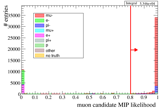
For example we can plot the muon candidate MIP likelihood before the PID cut and add an arrow to show which cut is made:
root [14] draw.SetTitleX("muon candidate MIP likelihood")
root [15] draw.Draw(data,mc,"selmu_likemip",50,0,1,"particle","accum_level>4")
root [16] draw.DrawCutLineVertical(200,true,"r")
Create file with event numbers for a given selection
There are function to extract the the event numbers for a given selection, which can be very useful to create skimmed files:
void PrintEventNumbers(TTree* tree, const std::string& cut, const std::string& file="", int refana=-1);
void PrintEventNumbers(
DataSample& sample,
const std::string& cut,
const std::string& file,
int refana=-1);
When calling the following function:
root [14] draw.PrintEventNumbers(default,"mu_mom>100 && mu_mom<200","events.list")
the file events.list is produced with the following content:
90200000,0,607
90200000,0,918
90200000,0,2142
90200000,0,2716
90200000,0,3312
90200000,0,3546
90200000,0,4746
90200000,0,6095
90200000,0,6187
where the first number is the run, the second subrun and the third the event number.