Description of examples
simple
This is a very simple example in which we learn how to simulate a trajectory (a set of measurements) and fit it to a given model.
By typing
> ./simple
you will see the usage
usage:
1. # events
2. verbosity (from 00000 to 77777). Digits: fitting, navigation, model, matching and simulation
3. X0 (rad length) in mm
4. dE/dx (energy loss rate) in MeV/mm
The number of events is mandatory but the rest are optional. The verbosity will help you in understanding the output. It contains five digits,
which correspond to different RecPack services. Basically you will start seing meaningful output from level 5 (from 0 to 4 are basically kept for warnings and errors).
The radiation length and energy loss rate to be simulated and used in the fitting can be also specified. By default no MS or energy loss are assumed.
So a possible way of running is
> ./simple 1000 0 425 -0.19
what means, 1000 events, with no RecPack output, 425 mm of radiation length and -0.19 MeV/mm of dE/dx, which are reasonable numbers for scintillator material.
The final output will be the setup at the beginning of the job and the fitting pulls at the end of the job.
complete
In this example, simulated trajectories with geant4 are read from a text file and fitted with the appropriate options. There are seven files available under the subdirectory data,
with and without magnetic field, multiple scattering and energy loss. Each of the files contain 1000 trajectories, all of them generated with the same initial parameters.
By typing
> ./complete
you will see the usage
usage:
1. # events
2. data file (from 1 to 7). Have a look at complete.cpp for different options
3. verbosity (from 00000 to 77777). Digits: fitting, navigation, model, matching and simulation
4. X0 (rad length) in mm. Data files generated with a value of 17.6 mm (iron)
5. dE/dx (energy loss rate) in MeV/mm. Data files generated with a value of -0.6 MeV/mm
It has one more parameter than the simple example, which is the data file to be used. This takes a value from 1 to 7. To have correct results for the files
with MS and/or energy loss, you should
specify the radiation length and the energy loss rate that was used for the simulation, which are 17.6 mm and -0.6 MeV/mm respectively.
So a possible way of running is
> ./complete 1000 4 0 17.6 -0.6
what means, 1000 events, run over the file 4, with MS, energy loss and magnetic field, with no RecPack output,
17.6 mm of radiation length and -0.6 MeV/mm of dE/dx.
The final output will be the setup at the beginning of the job and the fitting pulls at the end of the job.
For each event the results of the propagation and matching examples will be shown:
--------------- Example of propagation to a surface ------------------------
propagation: initial state = (-450.832702, 3.454282, 1799.995000, -0.248044, 0.000910, 0.001094)
---> length: 9900.7 propagated vector: (-5683.747749, 12.197876, 10000.000000, -1.241886, 0.001408, 0.001094)
--------------- Example of propagation to a length -------------------------
propagate to length ---> propagated vector = (-242.093105, 2.571153, 822.207621, -0.179400, 0.000897, 0.001094)
--------------- Example of matching from trajectory to measurement -------------------------
matching: chi2/ndf = 0.000570266
nd280_geom
This particular example explains how to use the ROOT geometry interface. Obviosuly this depends on ROOT and needs to include
the root part of the recpack library, which was not compiled by default.
All this is done automatically provided the ROOTSYS environment variable is set:
> export ROOTSYS="folder of ROOT in your system"
Then follow the standard procedure ("cmake ." + "make") to compile.
Before running this example
we should tell the system where the .root file with the geometry is. This is done by either setting manually the environment
variable ND280GEOM_EXAMPLE_DATA_DIR or running the script:
> source setup_nd280Geom.sh
Now you can run the example by typing
> ./DumpGeometry
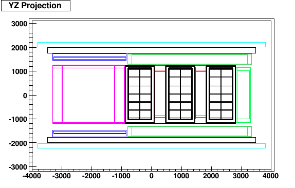
If everything goes well the ND280 geometry (the selected reduced set of volumes) will be dumped on the terminal and displayed on the screen.
This examples have many files/classes under the folder RecPack/examples/nd280_geom: