Getting started

Basic tutorial

ADerrors.jl is a package for error propagation and analysis of Monte carlo data. At the core of the package is the uwreal data type. It contains variables with uncertainties. In very simple cases this is just a central value and an error

julia> using ADerrors

julia> a = uwreal([1.0, 0.1], "Var with error") # 1.0 +/- 0.1
1.0 (Error not available... maybe run uwerr)

But it also supports the case where the uncertainty comes from Monte Carlo measurements

julia> # Generate some MC correlated data
       eta  = randn(1000);

julia> x    = Vector{Float64}(undef, 1000);

julia> x[1] = 0.0;

julia> for i in 2:1000
           x[i] = x[i-1] + eta[i]
           if abs(x[i]) > 1.0
               x[i] = x[i-1]
           end
       end

julia> b = uwreal(x.^2, "Random walk ensemble in [-1,1]")
0.33527917103774996 (Error not available... maybe run uwerr)

julia> c = uwreal(x.^4, "Random walk ensemble in [-1,1]")
0.2030633003289343 (Error not available... maybe run uwerr)

Correlations between variables are treated consistently. Each call to uwreal contains an ensemble ID tag. In the previous examples a has been measured on ensemble ID Var with error, while both b and c have been measured on ensemble ID Random walk ensemble in [-1,1]. Monte Carlo measurements with the same ID tag are assumed to be measured on the same configurations: b and c above are statistically correlated, while a will be uncorrelated with both b and c.

One can perform operations with uwreal variables as if there were normal floats

julia> d = 2.0 + sin(b)/a + 2.0*log(c)/(a+b+1.0)
0.9636821100662349 (Error not available... maybe run uwerr)

Error propagation is done automatically, and correlations are consistently taken into account. Note that once complex derived uwreal variables are defined, as for example d above, they will in general depend on more than one ensemble ID.

The message "(Error not available... maybe run uwerr)" in all the above statements suggests that newly defined uwreal variables do not know their error yet. In order to perform the error analysis of a variable, one should use the uwerr function

julia> uwerr(d);

julia> println("d: ", d)
d: 0.9636821100662349 +/- 0.09888273319053469

A call to uwerr will apply the $\Gamma$-method to MC ensembles. ADerrors.jl can give detailed information on the error of a variable (this requires that uwerr has been called)

julia> println("Details on variable d: ")
Details on variable d: 

julia> details(d)
0.9636821100662349 +/- 0.09888273319053469
 ## Number of error sources: 2
 ## Number of MC ids       : 1
 ## Contribution to error  :               Ensemble  [%]     [MC length]
  #                 Random walk ensemble in [-1,1]  93.32   1000
  #                                 Var with error   6.68            -

Here we can see that there are two ensembles contributing to the uncertainty in d. We recognize this as d being a function of both a (measured on ensemble Var with error), and b and c, measured on ensemble Random walk ensemble in [-1,1]. Most of the error in d comes in fact from ensemble Random walk ensemble in [-1,1].

Note that one does not need to use uwerr on a variable unless one is interested in the error on that variable. For example, continuing with the previous example

julia> global x = 1.0
1.0

julia> for i in 1:100
       	global x = x - (d*cos(x) - x)/(-d*sin(x) - 1.0)
       end

julia> uwerr(x)

julia> print("Root of d*cos(x) - x:" )
Root of d*cos(x) - x:
julia> details(x)
0.7227509415789974 +/- 0.04529112977875574
 ## Number of error sources: 2
 ## Number of MC ids       : 1
 ## Contribution to error  :               Ensemble  [%]     [MC length]
  #                 Random walk ensemble in [-1,1]  93.32   1000
  #                                 Var with error   6.68            -

determines the root on $d\cos(x) - x$ by using Newton's method, and propagates the error on d into an error on the root. The error on x is only determined once, after the 100 iterations are over. This feature is useful becase calls to uwerr are typically numerically expensive in comparison with mathematical operations of uwreal's.

Advanced topics

Errors in fit parameters

ADerrors.jl does not provide an interface to perform fits, but once the minima of the $\chi^2$ has been found, it can return the fit parameters as uwreal variables.

Here we are going to repeat the example of the package LsqFit.jl using ADerrors.jl for error propagation.

julia> using LsqFit, ADerrors

julia> # a two-parameter exponential model
       # x: array of independent variables
       # p: array of model parameters
       # model(x, p) will accept the full data set as the first argument `x`.
       # This means that we need to write our model function so it applies
       # the model to the full dataset. We use `@.` to apply the calculations
       # across all rows.
       @. model(x, p) = p[1]*exp(-x*p[2])
model (generic function with 1 method)

julia> # some example data
       # xdata: independent variables
       # ydata: dependent variable as uwreal
       xdata = range(0, stop=10, length=20);

julia> ydata = Vector{uwreal}(undef, length(xdata));

julia> for i in eachindex(ydata)
       	ydata[i] = uwreal([model(xdata[i], [1.0 2.0]) + 0.01*getindex(randn(1),1), 0.01], "Point "*string(i))
       	uwerr(ydata[i]) # We will need the errors for the weights of the fit
       end

julia> p0 = [0.5, 0.5];

We are ready to fit (xdata, ydata) to our model using LsqFit.jl

julia> # Fit the data with LsqFit.jl
       fit = curve_fit(model, xdata, value.(ydata), 1.0 ./ err.(ydata).^2, p0)
LsqFit.LsqFitResult{Array{Float64,1},Array{Float64,1},Array{Float64,2},Array{Float64,1}}([0.9940921904415403, 2.008415087061992], [0.026538818944554787, -0.241867285466274, 0.6135199223253021, -0.3544319056667286, 0.5428188151343266, -1.3285230976866003, -1.362823199632038, -1.1995557793263645, 0.7128553262789779, 1.801795500660672, -1.1687488707972047, -0.5890184345546259, -1.5258266588292717, 2.473887219653561, -0.7153828522840537, -0.5188281759352004, -0.9606748880562415, -0.2787993481410206, -1.9293117614323567, -0.3420774007941753], [100.00000000052196 0.0; 34.74756903895053 -18.180151062556398; … ; 5.452976891825284e-7 -5.13552724842633e-6; 1.8948003810366265e-7 -1.8836092224072973e-6], true, [10000.0, 10000.0, 10000.0, 10000.0, 10000.0, 10000.0, 10000.0, 10000.0, 10000.0, 10000.0, 10000.0, 10000.0, 10000.0, 10000.0, 10000.0, 10000.0, 10000.0, 10000.0, 10000.0, 10000.0])

In order to use ADerrors.jl we need the $\chi^2$ function.

julia> # ADerrors will need the chi^2 as a function of the fit parameters and
       # the data. This can be constructed easily from the model function above
       chisq(p, d) = sum( (d .- model(xdata, p)) .^2 ./ 0.01^2)
chisq (generic function with 1 method)

A call to fit_error will return the fit parameters as a Vector{uwreal} and also the expected value of the $\chi^2$ as a Float64

julia> # This is error propagation with ADerrors.jl
       (fitp, cexp) = fit_error(chisq, coef(fit), ydata);

julia> println("Fit results: \n
       	     chi^2 / chi^2_exp: ", sum(fit.resid .^2), " / ", cexp, " (dof: ", dof(fit), ")")
Fit results: 

	     chi^2 / chi^2_exp: 25.453732581342578 / 18.000000000000004 (dof: 18)

julia> # fitp are the fit parameters in uwreal
       # format. One can use them as any other uwreal
       # For example to determine the main contribution
       # to its uncertainty
       for i in 1:2
       	uwerr(fitp[i])
       	print("Fit parameter: ", i, ": ")
       	details(fitp[i])
       end
Fit parameter: 1: 0.9940921904415403 +/- 0.009931043850361709
 ## Number of error sources: 20
 ## Number of MC ids       : 0
 ## Contribution to error  :               Ensemble  [%]     [MC length]
  #                                        Point 1  98.54            -
  #                                        Point 2   0.54            -
  #                                        Point 3   0.47            -
  #                                        Point 4   0.32            -
  #                                        Point 5   0.10            -
  #                                        Point 6   0.02            -
  #                                        Point 7   0.00            -
  #                                        Point 8   0.00            -
  #                                        Point 9   0.00            -
  #                                       Point 10   0.00            -
  #                                       Point 11   0.00            -
  #                                       Point 12   0.00            -
  #                                       Point 13   0.00            -
  #                                       Point 14   0.00            -
  #                                       Point 15   0.00            -
  #                                       Point 16   0.00            -
  #                                       Point 17   0.00            -
  #                                       Point 18   0.00            -
  #                                       Point 19   0.00            -
  #                                       Point 20   0.00            -
Fit parameter: 2: 2.008415087061992 +/- 0.04552802718661561
 ## Number of error sources: 20
 ## Number of MC ids       : 0
 ## Contribution to error  :               Ensemble  [%]     [MC length]
  #                                        Point 2  50.59            -
  #                                        Point 3  28.48            -
  #                                        Point 1  10.62            -
  #                                        Point 4   8.12            -
  #                                        Point 5   1.79            -
  #                                        Point 6   0.34            -
  #                                        Point 7   0.06            -
  #                                        Point 8   0.01            -
  #                                        Point 9   0.00            -
  #                                       Point 10   0.00            -
  #                                       Point 11   0.00            -
  #                                       Point 12   0.00            -
  #                                       Point 13   0.00            -
  #                                       Point 14   0.00            -
  #                                       Point 15   0.00            -
  #                                       Point 16   0.00            -
  #                                       Point 17   0.00            -
  #                                       Point 18   0.00            -
  #                                       Point 19   0.00            -
  #                                       Point 20   0.00            -

Missing measurements

ADerrors.jl can deal with observables that are not measured on every configuration, and still take correctly the correlations/autocorrelations into account. Here we show an extreme case where one observable is measured only in the even configurations, while the other is measured on the odd configurations.

julia> using ADerrors, Plots

julia> pgfplotsx();

julia> # Generate some correlated data
       eta  = randn(10000);

julia> x    = Vector{Float64}(undef, 10000);

julia> x[1] = 0.0;

julia> for i in 2:10000
           x[i] = x[i-1] + 0.2*eta[i]
           if abs(x[i]) > 1.0
               x[i] = x[i-1]
           end
       end

julia> # x^2 only measured on odd configurations
       x2 = uwreal(x[1:2:9999].^2,  "Random walk in [-1,1]", collect(1:2:9999),  10000)
0.3251681660845364 (Error not available... maybe run uwerr)

julia> # x^4 only measured on even configurations
       x4 = uwreal(x[2:2:10000].^4, "Random walk in [-1,1]", collect(2:2:10000), 10000)
0.19540757268935874 (Error not available... maybe run uwerr)

the variables x2 and x4 are normal uwreal variables, and one can work with them as with any other variable. Note however that the automatic determination of the summation window can fail in these cases, because the autocorrelation function with missing measurements can be very complicated. For example

julia> rat = x2/x4 # This is perfectly fine
1.664050996639006 (Error not available... maybe run uwerr)

julia> try # Use automatic window: might fail!
           uwerr(rat)
       catch e
           println("Automatic window fails")
       end
ID's with negative tau_int: 
     Random walk in [-1,1]
Automatic window fails

In this case uwerr complains because with the automatically chosen window the variance for ensemble with ID "Random walk in [-1,1]" is negative. Let's have a look at the normalized autocorrelation function

julia> iw = window(rat, "Random walk in [-1,1]")
2

julia> r  = rho(rat, "Random walk in [-1,1]");

julia> dr = drho(rat, "Random walk in [-1,1]");

julia> plot(collect(1:100),
       	r[1:100],
       	yerr = dr[1:100],
       	seriestype = :scatter, title = "Chosen Window: " * string(iw), label="autoCF")
Plot{Plots.PGFPlotsXBackend() n=1}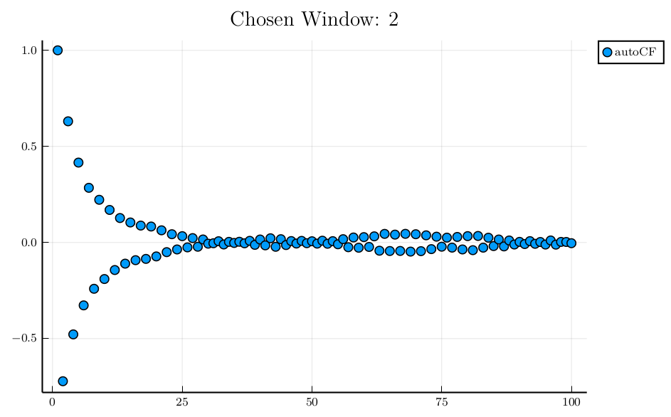

The normalized autocorrelation function is oscillating, and the automatically chosen window is 2, producing a negative variance! We better fix the window to 50 for this case

julia> wpm = Dict{String, Vector{Float64}}()
Dict{String,Array{Float64,1}}()

julia> wpm["Random walk in [-1,1]"] = [50.0, -1.0, -1.0, -1.0]
4-element Array{Float64,1}:
 50.0
 -1.0
 -1.0
 -1.0

julia> uwerr(rat, wpm) # repeat error analysis with our choice (window=50)

julia> println("Ratio: ", rat)
Ratio: 1.664050996639006 +/- 0.025169502432762753

After a visual examination of the autocorrelation function and a reasonable choice of the summation window, the error in rat is determined. Note however that it is very difficult to anticipate which observables will have a strange autocorrelation function. For example the product of x2 and x4 shows a reasonably well behaved autocorrelation function.

julia> prod = x2*x4
0.06354032205042952 (Error not available... maybe run uwerr)

julia> uwerr(prod)

julia> println("Product: ", prod)
Product: 0.06354032205042952 +/- 0.0044984614962039595

julia> iw = window(prod, "Random walk in [-1,1]")
72

julia> r  = rho(prod, "Random walk in [-1,1]");

julia> dr = drho(prod, "Random walk in [-1,1]");

julia> plot(collect(1:2*iw),
       	r[1:2*iw],
       	yerr = dr[1:2*iw],
       	seriestype = :scatter, title = "Chosen Window: " * string(iw), label="autoCF")
Plot{Plots.PGFPlotsXBackend() n=1}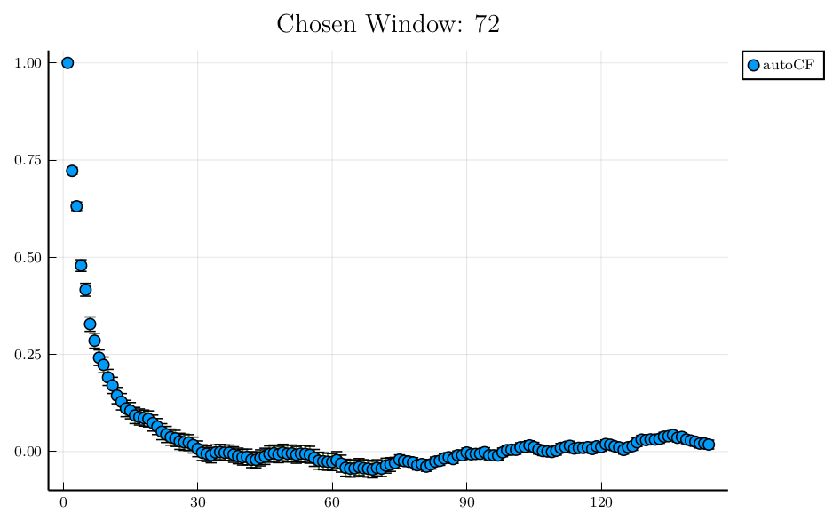

In general error analysis with data with arbitrary gaps is possible, and fully supported in ADerrors.jl. However in cases where many gaps are present, data analysis can be tricky, and certainly requires some care.

BDIO Native format

ADerrors.jl can save/read observables (i.e. uwreal's) in BDIO records. Here we describe the format of these records.

All observables are stored in a single BDIO record of type BDIO_BIN_GENERIC. The record has the following data in binary little endian format

• mean (Float64): The mean value of the observable.
• neid (Int32): The number of ensembles contributing to the observable.
• ndata (Vector{Int32}(neid)): The length of each ensemble.
• nrep (Vector{Int32}(neid)): The number of replica of each enemble.
• vrep (Vector{Int32}): A vector with length the number of replica that contains the number of measurements in each replica.
• ids (Vector{Int32}(neid)): The ensemble numeric ID's.
• nt (Vector{Int32}(neid)): Half the largest replica of each ensemble.
• zero (Vector{Float64}(neid)): just neid zeros.
• four (Vector{Float64}(neid)): just neid fours.
• delta (Vector{Float64}): The fluctuations for each ensemble.
• name (NULL terminated String): A description of the observable.
• ID tags: A list of neid tuples (Int32, String) that maps each numeric ID to an ensemble tag. All strings are NULL terminated.
• Replica details: neid times the following information:
  • First an Int32 wiht the numeric ID tag of the ensemble.
  • Then a Vector{String} that contains the replica names.
  • Finally a Vector{Int32} that contains the the configuration index where each measurement has been performed.

It is encouraged that the first record of the BDIO file is an ASCII human readable record explaining the estructure of the file. By convention, this record has user info=1. An example file containing the